
LiDAR-Based SLAM (Click Here!)
Full code can be provided upon request
Introduction
In the realm of robotics, precise environment perception and navigation are crucial for a wide range of applications, from autonomous vehicles to robots in complex environments. The primary challenge in achieving this is the process known as Simultaneous Localization and Mapping (SLAM), which involves both mapping an environment and determining the robot’s position within that map. This project addresses this challenge by leveraging multiple sensors: IMUs, Encoders, Lidar, and RGBD cameras.
The approach starts with Dead Reckoning, which uses IMU and Encoder data to estimate the robot’s position and orientation, although this method is prone to cumulative errors. To improve accuracy, the Iterative Closest Point (ICP) algorithm is applied to Lidar data, refining the trajectory estimate. Further optimization is achieved using factor graphs, which incorporate all sensor data into a unified framework to enhance precision. The project also generates two types of maps: Occupancy Grid maps, which represent the environment as a grid of obstacles, and Texture maps, which add visual detail by incorporating data from the RGBD camera.
Problem Formulation
What We Have
The project uses a differential-drive robot equipped with encoders, an IMU, a 2-D Lidar, and an RGBD camera. The encoders track wheel rotations, the IMU provides yaw rate data, the Lidar measures distances to obstacles, and the RGBD camera captures both color and depth images.
Figure 1: Differential-drive robot equipped with sensors. 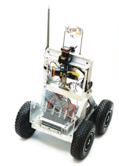
Motion Model
The robot’s motion is modeled using a differential-drive kinematic model, which calculates the robot’s position and orientation over time based on encoder and IMU data.
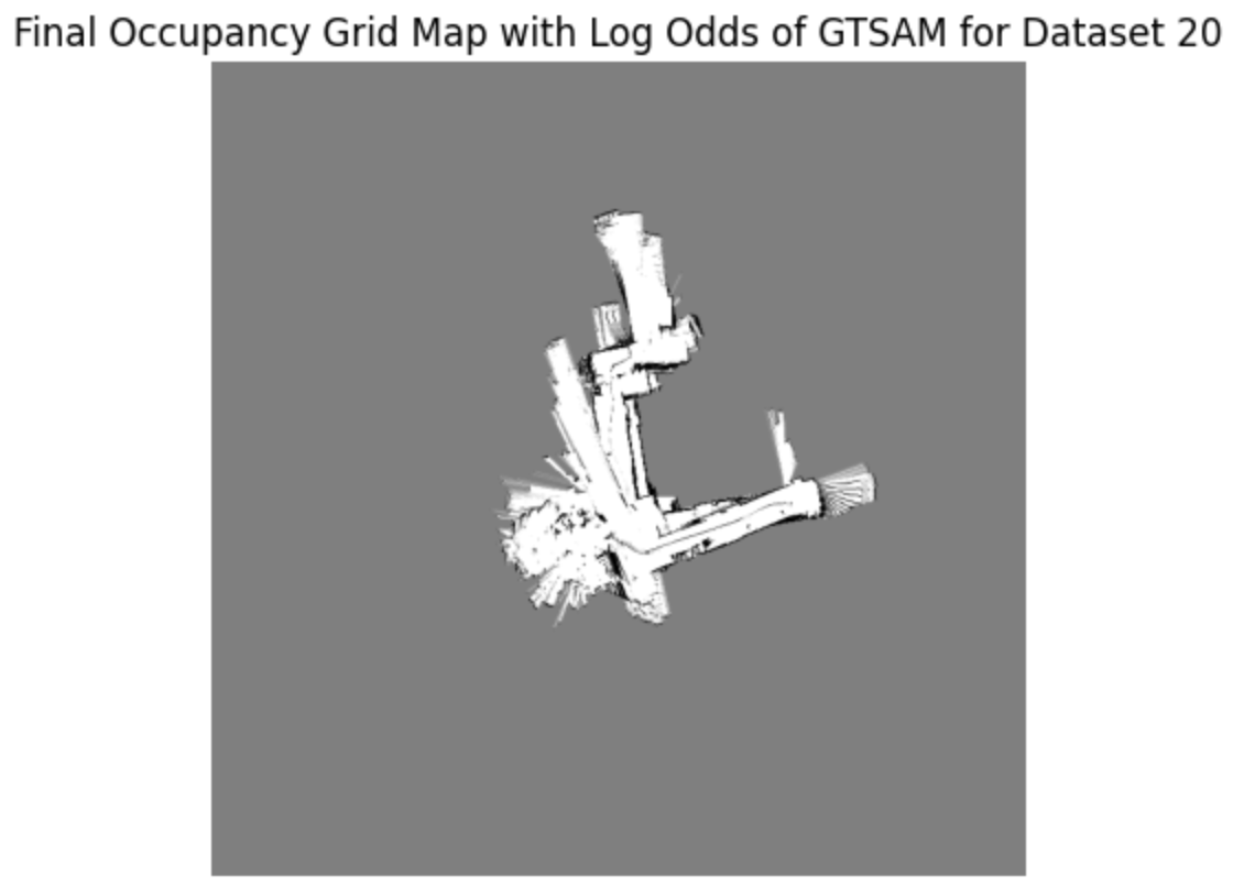
Occupancy Grid Map
The occupancy grid map represents the environment as a grid where each cell can be occupied, free, or unknown. The map is updated using sensor measurements, with the occupancy state of each cell estimated over time based on the robot’s trajectory and sensor data.
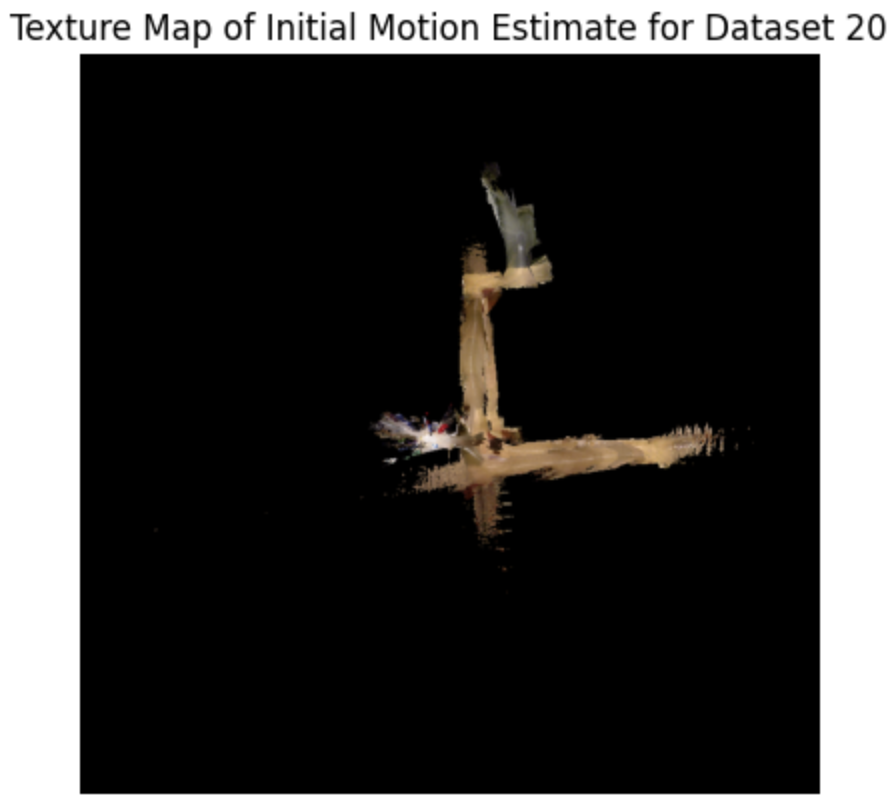
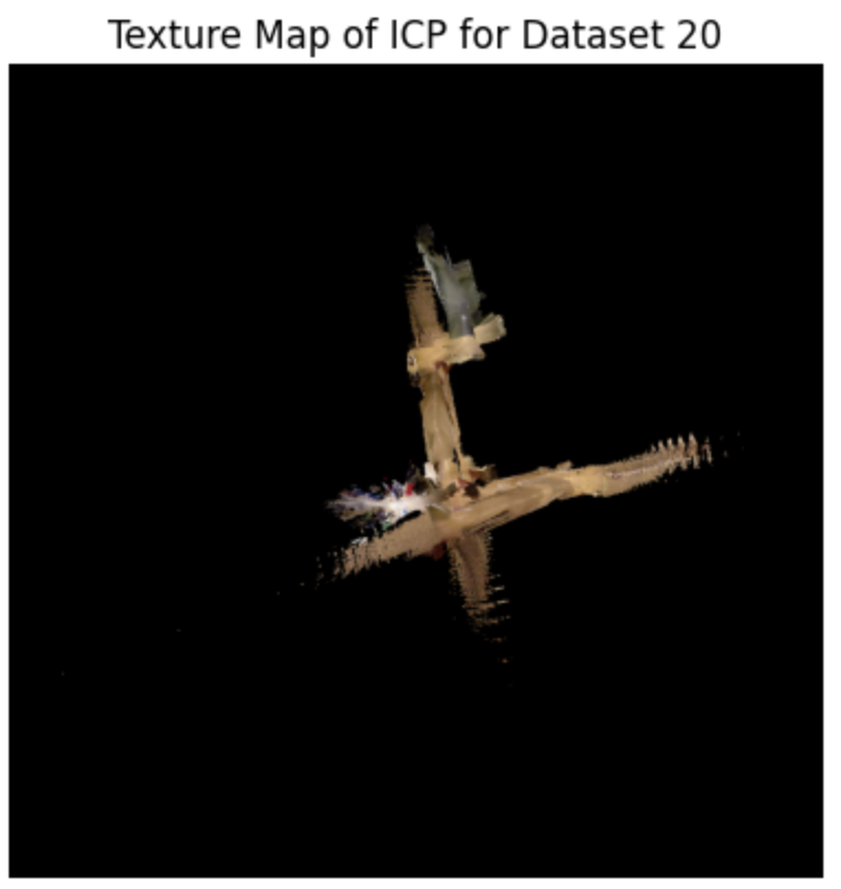
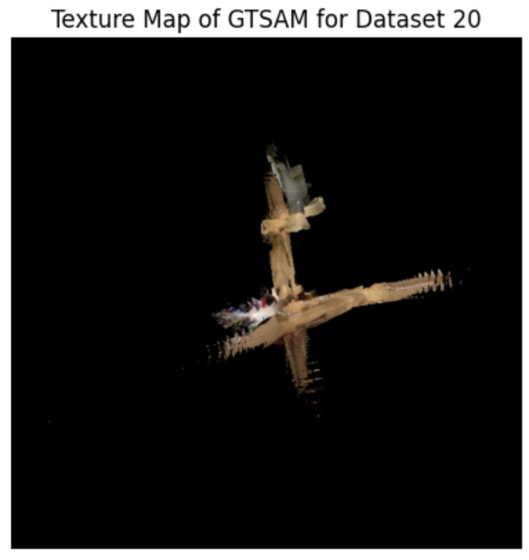
Texture Map
The texture map enhances the occupancy grid by adding color information from the RGBD camera, providing a more detailed visual representation of the environment.
Factor Graph
Factor graphs are used to optimize the robot’s trajectory estimation by incorporating constraints from odometry and loop closures. The GTSAM framework is employed to construct and solve the factor graph, refining the robot’s pose estimates.
Technical Approach
Preliminary
The data from the various sensors is synchronized using their timestamps, ensuring that all data points correspond to the same time frame.
Dead Reckoning
Dead Reckoning combines IMU and Encoder data to estimate the robot’s trajectory over time. This involves calculating the robot’s velocity and using a motion model to predict its position and orientation.
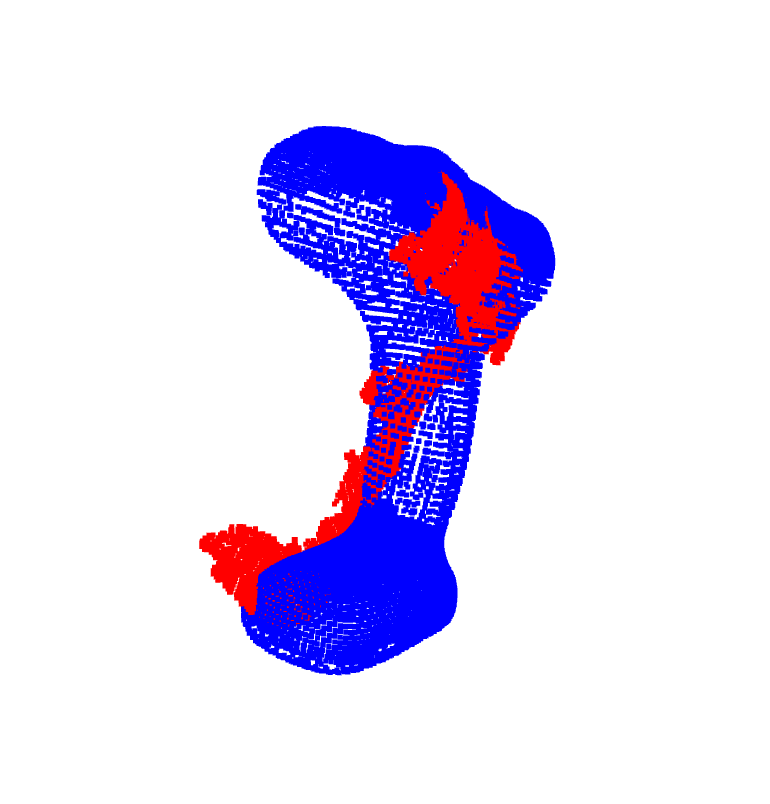
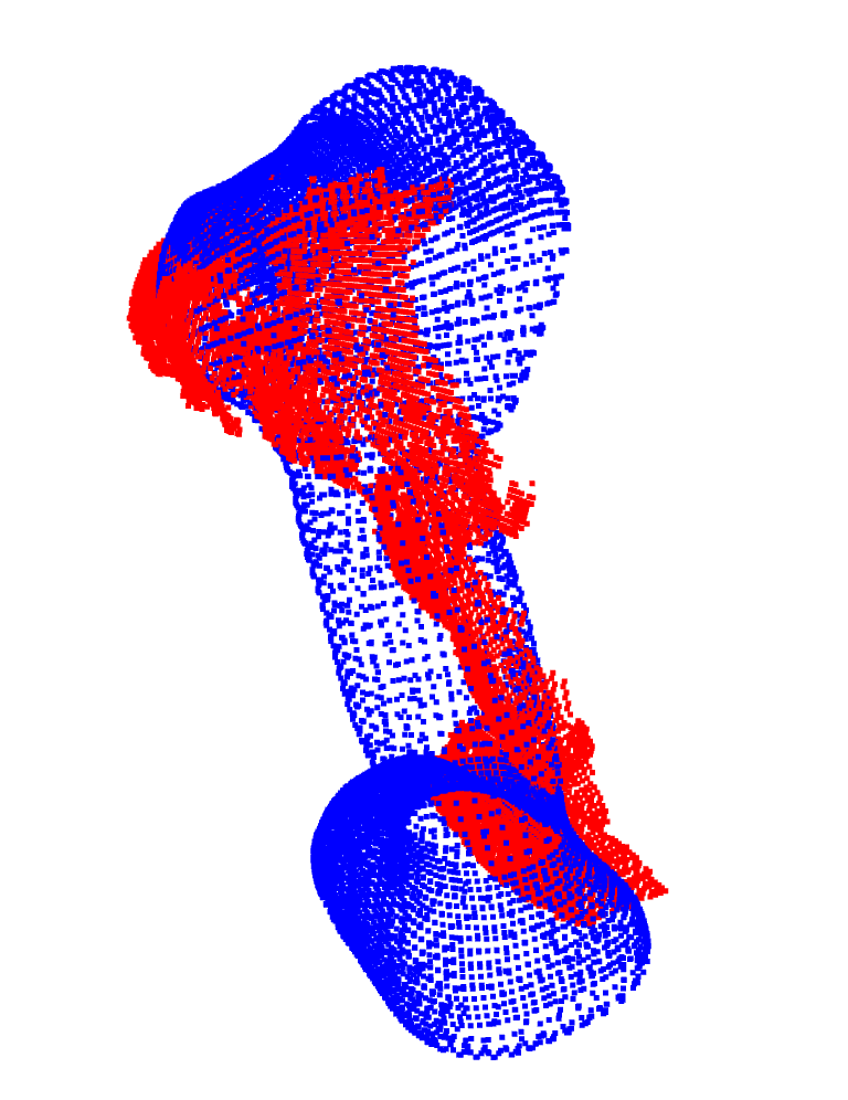
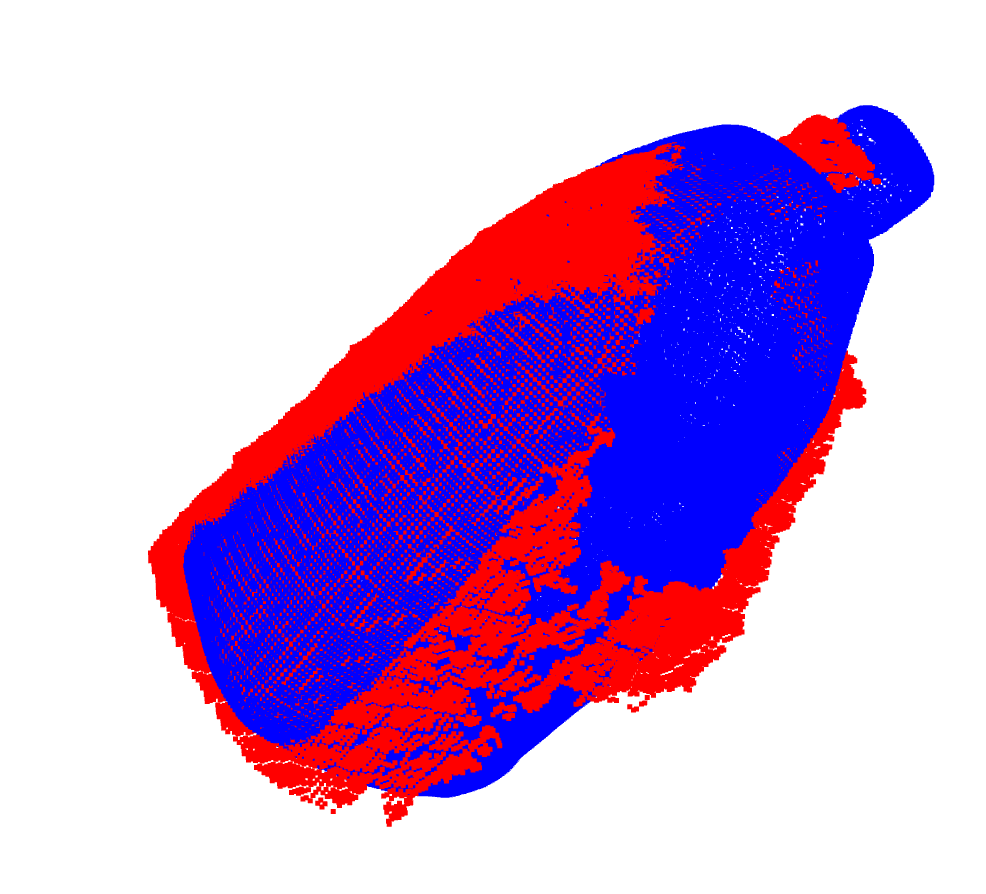
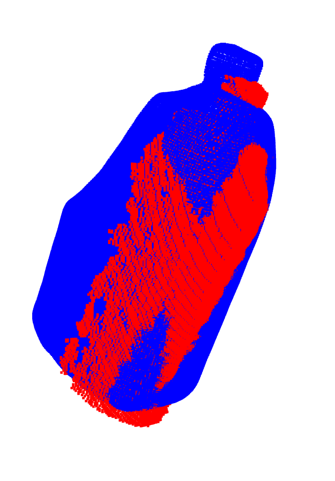
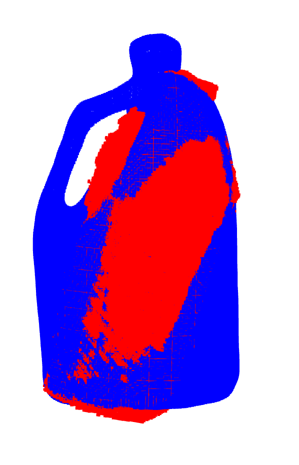
Scan Matching (ICP)
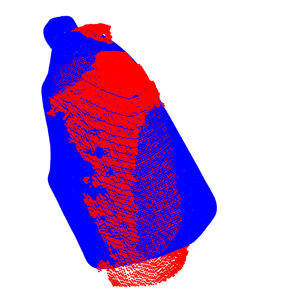
ICP is used to align Lidar scans and refine the robot’s trajectory. This process involves calculating the relative transformation between consecutive robot poses using Lidar data and the Kabsch algorithm.
Figure 2: Drill scan matching for warm-up.
 |  |
 | 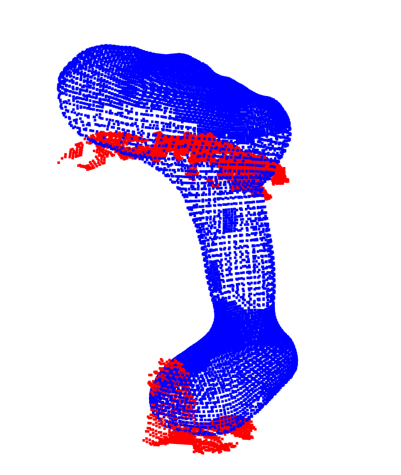 |
Figure 3: Liquid container scan matching for warm-up.
 |  |
 |  |
Occupancy Grid Mapping
The environment is discretized into a grid, and Lidar data is used to update the occupancy state of each cell. The Bresenham2D algorithm is applied to trace the path of sensor rays, updating the map based on the detected obstacles.
Texture Mapping
Depth information from the RGBD camera is combined with color data to create a texture map. This involves transforming pixel coordinates from the camera frame to the world frame and mapping RGB data onto the 3D points.
Factor Graphs and Loop Closure
A factor graph is constructed using the GTSAM framework to optimize the robot’s trajectory. Loop closure constraints are added based on Lidar measurements to correct for drift in the trajectory.
Results
Dead Reckoning
The initial trajectory estimates from Dead Reckoning are reasonable and are used to generate rough maps of the environment by projecting Lidar scans.
Figure 4: Initial motion estimate. 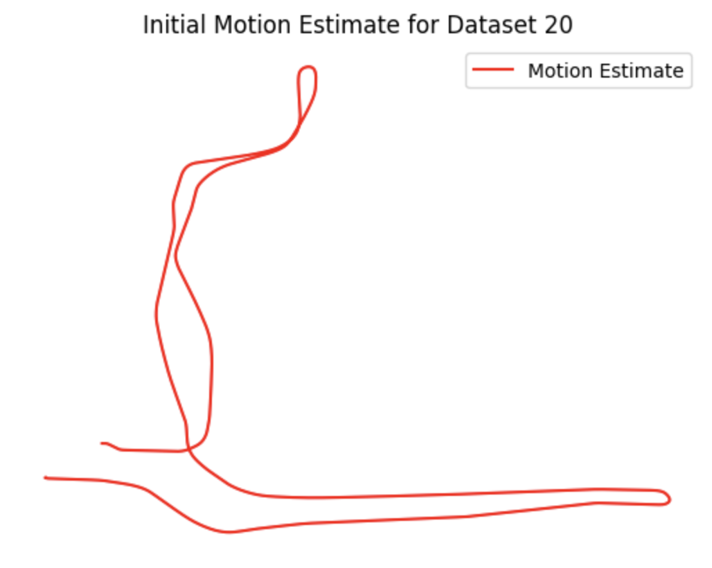
Figure 5: Projected Lidar scans from initial motion estimate. 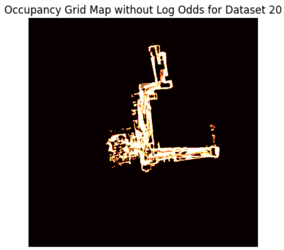
Scan Matching (ICP)
ICP results show that while it improves the alignment of point clouds, it does not perform as well as the motion model in terms of overall trajectory estimation.
Figure 6: Initial motion estimates (Red) vs ICP (Blue). 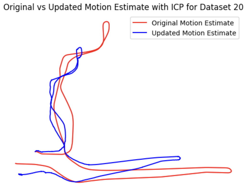
Occupancy Grid Mapping
The occupancy grid maps generated from the motion model, ICP, and GTSAM show that the motion model provides the best estimate, with GTSAM offering slight improvements.
Figure 7: Occupancy grid map with initial motion estimate, ICP, and GTSAM.
 |  |  |
Texture Mapping
Similar to the occupancy grid maps, the texture maps indicate that the motion model gives the best results, with GTSAM slightly improving the map quality.
Figure 8: Texture grid map with initial motion estimate, ICP, and GTSAM for Dataset 20.
 |  |  |
Factor Graphs and Loop Closure
Factor graph optimization with GTSAM shows a slight improvement over ICP, but the motion model still provides the most accurate estimates.
Figure 9: Initial motion, ICP, and GTSAM trajectories. 
Conclusion
This project successfully implemented SLAM using a variety of sensors and advanced techniques like ICP and factor graph optimization. The results demonstrated that while these methods improved trajectory estimation and mapping, the motion model remained the most reliable approach. Future work could explore the use of the Extended Kalman Filter for similar objectives, potentially offering a more sophisticated alternative.